Using 3LC in CV Model Training

This document provides examples and recommendations for integrating the 3LC tool into model training notebooks for computer vision models. The focus will be on semantic segmentation, using the SegFormer model from Hugging face.

Resources for beginners

Some useful resources can be found here for beginners. These resources were provided by 3LC.

• Documentation: 3LC Documentation
• Architecture: 3LC Customer Managed Architecture
• Tutorials: Tutorials
• Example Notebooks: Example Notebooks
• GitHub: 3LC GitHub _ Example Notebooks & Tutorials
• YouTube Channel: 3LC YouTube Channel

Tool Implementation

The 3LC tool is implemented in multiple pieces/containers which essentially include the 3LC Object service and the 3LC Dashboard service.

• 3LC Object Service: provides R/W access to training data and metrics
• 3LC Dashboard Service: serves the 3LC Dashboard web-application

Connecting the dashboard to the object service

For our implementation, the Dashboard service was implemented on our KubeFlow ecosystem as a standalone application that will connect to the object service that can be specified in the URL setting of the dashboard settings menu (see Figure 1).

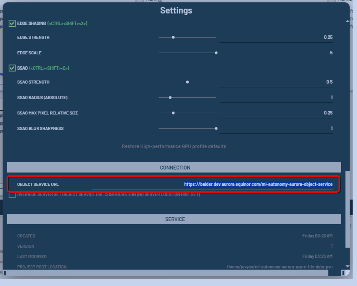Figure 1: Set the URL in the Object Service URL field of the Dashboard's menu.

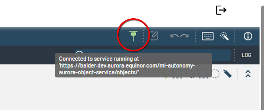Figure 2: Confirming healthy connection to the object service.

Validating dashboard connection to object service

One way to check and confirm that the dashboard is connected to the object service is to create a simple table with the Jupyter Notebook and confirm that it can be seen in the dashboard.

Example:

import tlc

data = {
    "COLUMN": [0, 11, 22, 33, 44, 55, 66]
}

table = tlc.Table.from_dict(
    data,
    project_name="Equinor_TableTest",
    table_name="TestTable2"
)

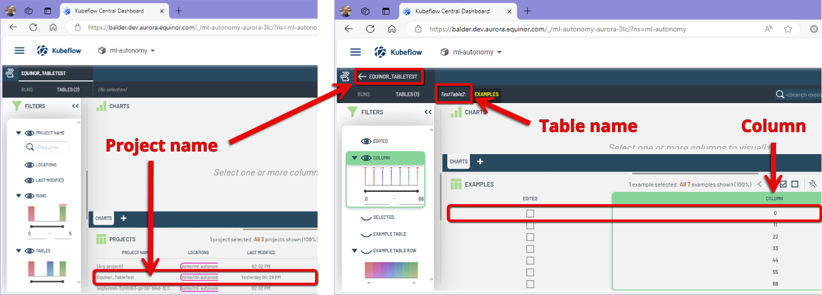Figure 3: Confirming table creation in dashboard with project name, table name, and numerical data column.

note

We implemented an object server that stores data in the same volume as the workspace/processing notebook for easy read/write access when using the 3LC tool. This is done via an Azure Volume mounted to the workspace (Jupyter Notebook) and linked to the dashboard through its hosted object service.

SegFormer Model

The implementation is illustrated in an example notebook where the small size SegFormer model 'mit-b0' is trained on a dataset of images of subsea pipelines featuring various objects.

This dataset consists of 1000 synthetically generated images depicting different pipeline configurations with anodes, mines, rocks, and debris on the subsea floor.

The reference tutorial we implemented for our exercise can be found here:

• Fine-tune Hugging Face SegFormer on custom dataset

Editing Annotation Files

On the dashboard, it is possible to tweak the segmentation mask to make edits. You can use the toolbar to edit the mask as needed.

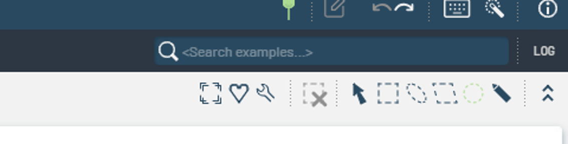Figure 4: Dashboard toolbar used for editing the segmentation mask.

How to edit the mask

1. In the following image (Figure 5), let's edit the mask so that:
   • the anode object is consolidated into one solid object rather than multiple fragments,
   • and let's remove the small rock in the far left.

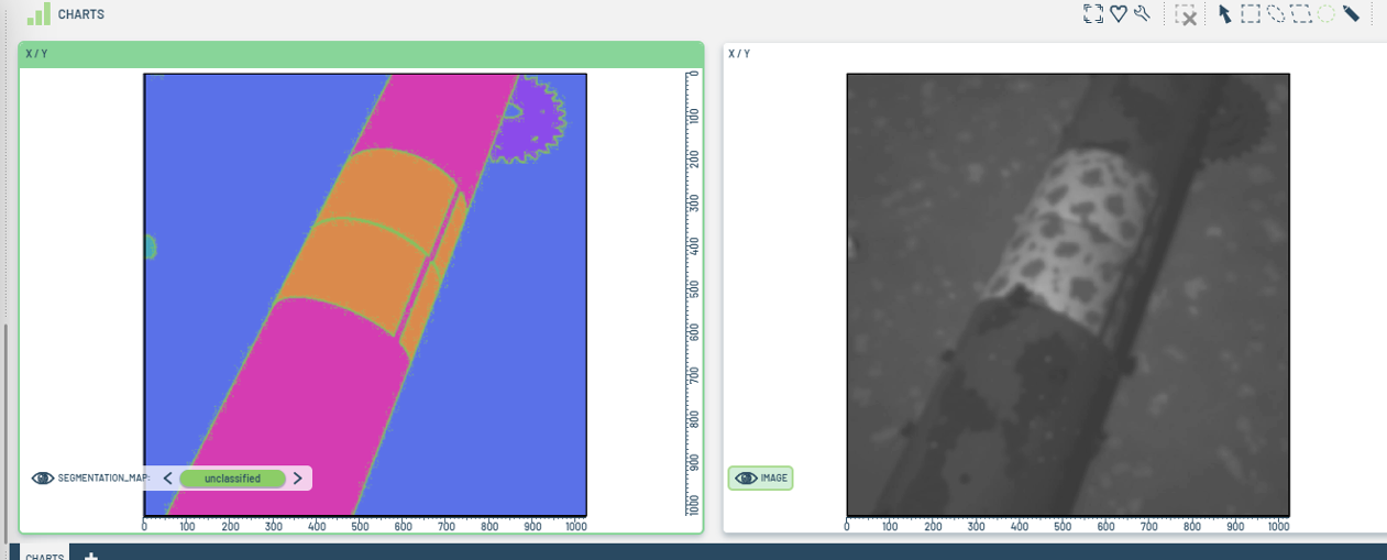Figure 5: Sample of image mask.

2. We can use a box tool to cover the rock with a rectangular seabed object. You can make the selection using the object menu from the mask image:

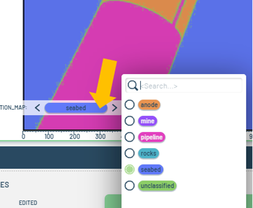Figure 6: Object menu from the mask image.

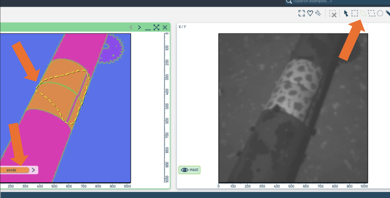Figure 7: Tool selection.

3. After making the edits, we must confirm and commit the changes to save the edited masks into PNG files.
   • Observe the yellow notification in the upper menu button; it shows the count of pending edits.
   • Open the menu, add any necessary comments, and then commit the changes to finalize.

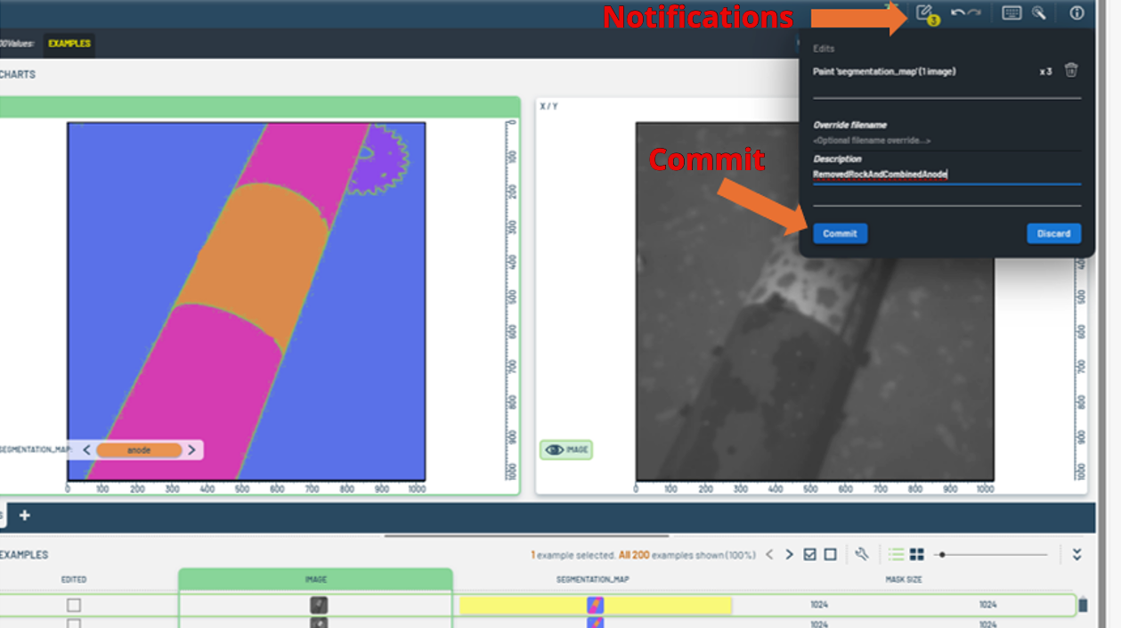Figure 8: Notifications & commit button

How to use the modified masks to train your model

1. To use the modified masks for training your model, check the tables view and note the lineage column displaying the edits' progression and their references.

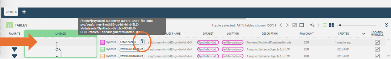   Figure 9: Table view with lineage column.

2. In the table view, you can copy the path to where the revised data table object is located. This path can be utilized in the notebook to directly read the data tables while preparing datasets for training.

   note

   Go to the tlc.core.objects.table documentation for details on reading data tables with 3LC.

   Here are a some methods that you can use:

   • Reading using a reference path
   • Using the overwrite argument
   • Reading from a URL
   • Reading the latest version

Editing Training Weights

If needed, the image dataset can be assigned weights to prioritize specific subsets. For instance, if the model underperforms on certain images, those images can be given higher weights. With higher weights, the sampler will prioritize these images during model training over others in the dataset.

In another scenario, if the model's performance is poor on specific objects within the image set, we can develop metrics focusing on the model's performance on those particular objects.

The training process utilizes the weights column of the 3LC table to sample data (images) from the train set. Initially, all weights are set to 1, unless changed by the user.

Adjusting weights for specific images

To adjust weights for specific images directly in the dashboard using the weights column, do the following:

1. Click the wrench settings icon and use the settings menu from the Run to enable the Weight column.

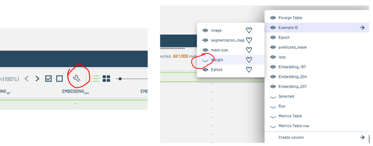   Figure 10: Enabling the Weight column.

2. Edit the Weight column as desired.

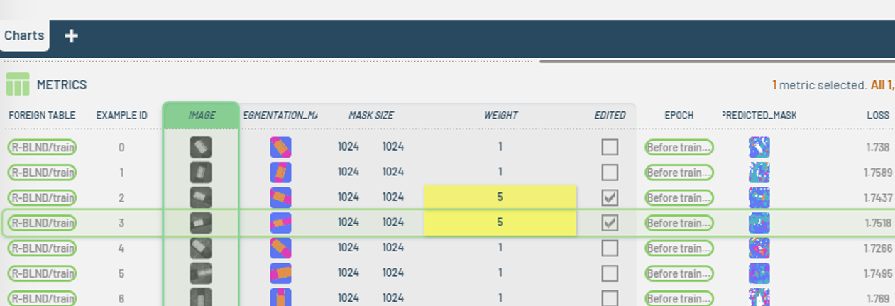   Figure 11: Editing the Weight column.

3. A notification will show up in the top menu reflecting how many edits are pending for commit.

   
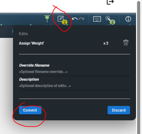
   Figure 12: Edits pending commit.

4. You can enter names and descriptions before committing changes, which will push the new weights to a fresh URL for a new training session.

note

• Depending on the edits to the training or validation sets, a new URL will be generated, available in the tables view of the dashboard.
• The table view shows the dataset lineage, including sources and edits.
• You can use the URL column to copy the direct address for the edited tables and set them up for retraining.
• Heavier weights will make the sampler focus more on those images; however, weights on the validation set don't affect model training.

Applying weights based on calculated performance metrics

1. Follow the process from the previous section to show the Weight column in a specific Run view.

2. Next, update the entire weight column using a calculated metric by dragging and dropping it into the weight column header.

3. In this instance, we'll assign the loss to the weight column.

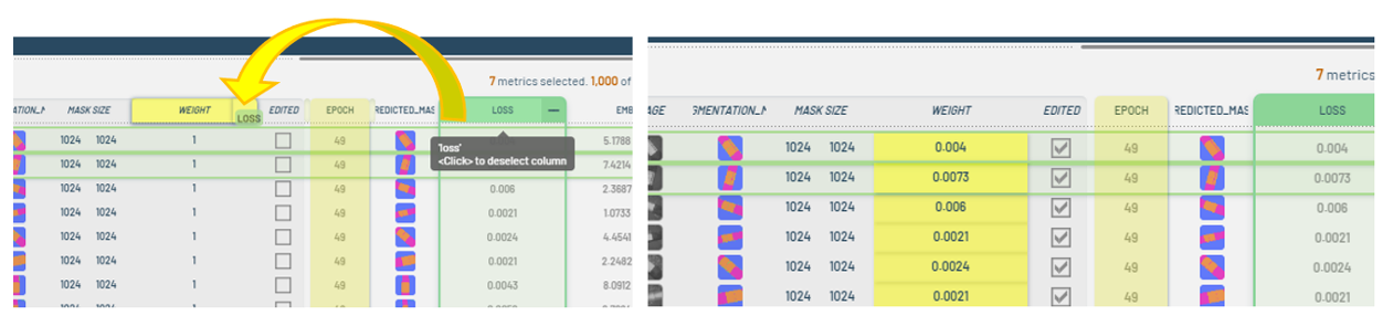   Figure 13: Assigning loss to weight.

   note

   • It is crucial to examine the distribution of the metric, which can be done using the vertical filter panel, and determine whether it needs to be retained or modified before applying it.
   • For instance, if the metric ranges from [0.01 - 10], directly using the weight could lead to some images being weighted 1000 times more than others, resulting in imbalance issues. To mitigate this in the given example, you could add 5 to the metric column before assigning it to 'weight'.
   • This adjustment would mean the weight ranges from [5.01 - 15], reducing the disparity so that, at most, some images are only weighted three times more than others.

Performing mathematical operations on table columns

1. You can perform mathematical operations on the table's columns by right-clicking the desired column and creating virtual columns. This action will add a calculated column immediately to the right of the original one.

   
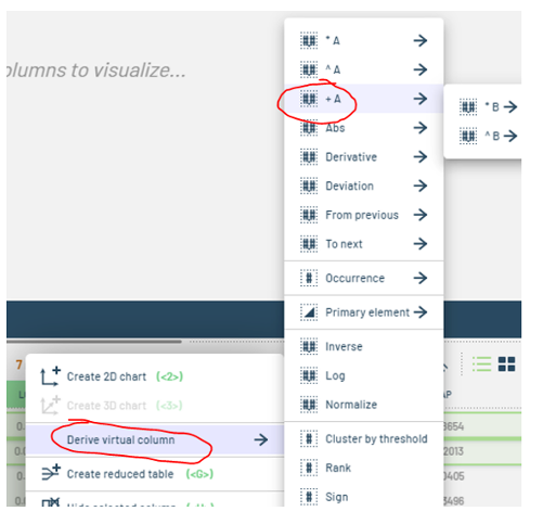
   Figure 14: Creating a virtual column.

2. To modify this newly generated column, right-click it and choose from the options shown in the subsequent screenshots to adjust the default adder, multiplier, power, or any other constants applied to the virtual column.

   
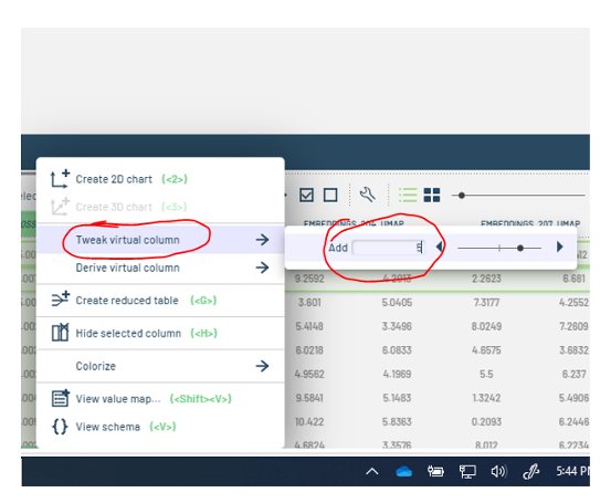
   Figure 15: Editing a virtual column.

Balancing Training by Adjusting Dataset Weights to Object Content

In this section, we're dealing with a class-imbalanced dataset for training a SegFormer model.

Dataset imbalance

• The dataset includes simulated subsea pipeline images with various components, degradations, and camera views.
• A specific class, representing gas leaks via bubbles, appears in only a few images.
• This imbalance might cause the trainer to overlook this class, affecting detection performance.

Solution

Here is solution using 3LC tools is to assign higher weights to images containing the leak/bubble class.

To carry out the solution, we can do the following:

• By filtering the raw data in table view, we can identify how often the object appears among all images. For instance, out of 1082 images, only 215 include leaks, resulting in a ratio of about 1/5.
• To rebalance, we might give leak images a weight of 5, while others remain at 1.
• Considering camera variations, we could also weigh CameraForward leak images at 4 and TopDown ones at 6.

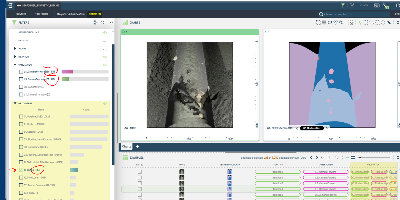Figure 16: Filtering

Remove Images from Training or Validation Datasets

You can modify the tables on the 3LC dashboard to remove rows of images that you don't want in the training or validation sets.

note

This won't physically delete the files from the drive; it will simply exclude those images during model training and metric evaluation.

How to remove images

To remove images:

1. Select the image, or rows of images to be deleted, and right-click.
2. Select Delete table rows (See Figure 17).

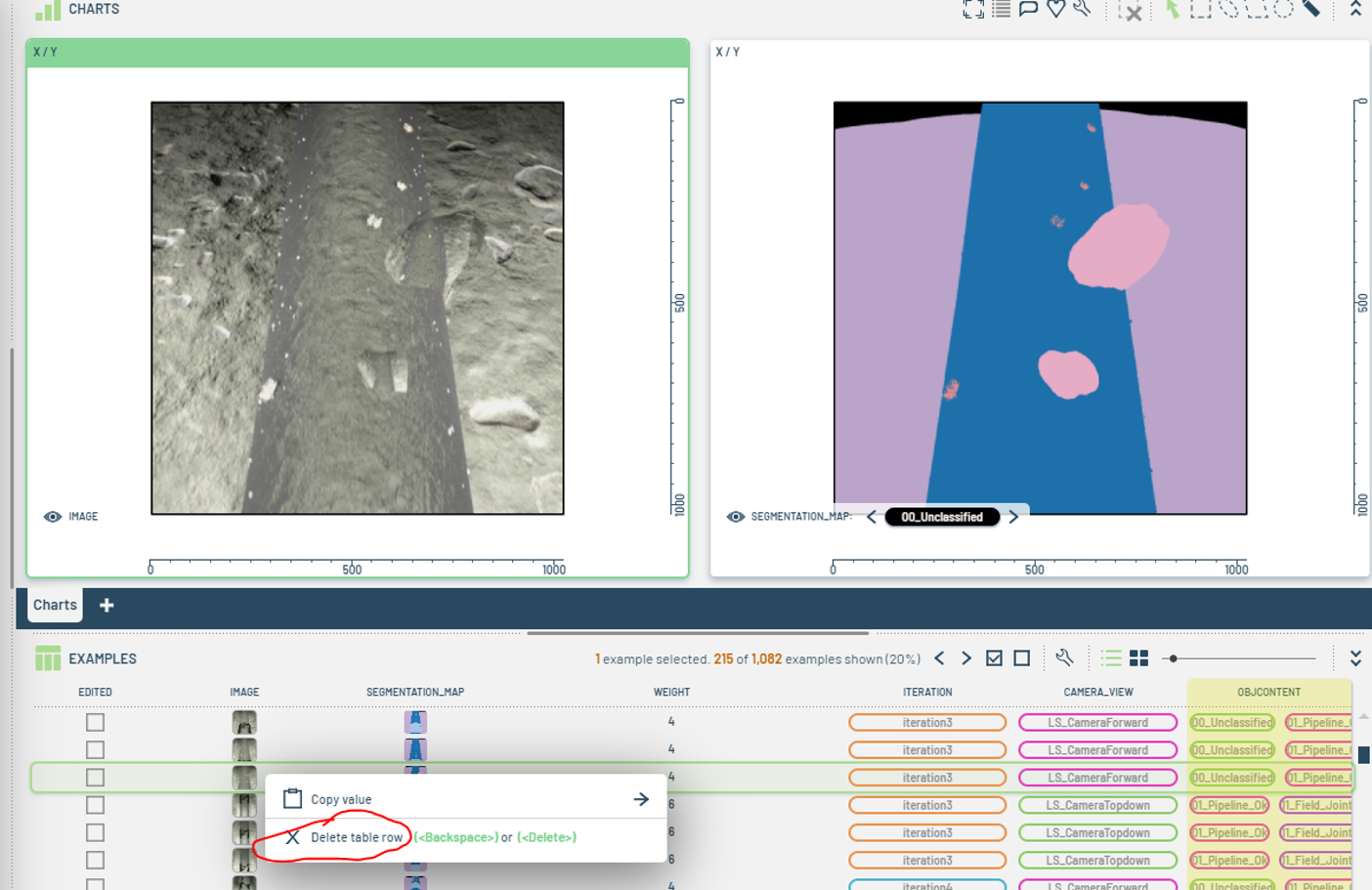Figure 17: Removing images.

tip

If you prefer to keep the images in the training tables but still need metrics calculated for them, you can leave the rows intact and set their weight to zero so that the sampler ignores them for training purposes.

Extended Table Creation

In our training examples, we considered multiple variables to construct a comprehensive dataset that reflects various conditions, views, sceneries, brightness levels, environments, and ingredients.

To facilitate the manipulation of image tables, additional columns can be created to incorporate specific metadata into the dataset. This approach aids in setting filters, examining statistics, or simply selecting objects of interest.

Example

For instance, we developed an extended table that builds on the baseline table, which includes only the image path, segmentation mask, and image size. The extended table adds columns for Camera View, the Iteration during which the raw images were generated, and an Object Content column that lists different object codes present in the image based on annotations from the mask.

Benefits

This method helps analyze the data more objectively, such as determining which classes are prevalent and how to re-weight the images to rebalance them based on content. It also allows organizing the dataset by categories like camera view and identifying common denominators among the images to decide whether further edits or additional views and tweaks are necessary.

Creating extended table columns

To create these extended table columns, refer to a notebook file where the table creation occurs using the tlc.TableWriter method. For example:

• Create Custom Table - 3LC Tutorial
• Per Bounding Box Luminosity Calculation - 3LC Example Notebooks

Referencing the table

This process builds upon the referenced baseline table by appending the new columns as explained. Ensure you reference this new table by its URL when training a new model or collecting metrics, so the Run results will display the added columns.

Evaluation with a SegFormer Training Exercise

For this assessment, a synthetic dataset comprising 17 objects of interest was utilized. To evaluate incremental improvements using the 3LC tool, we performed the following training runs:

• Run 0: Baseline (with mit-b0)
• Run 1: Cleaned dataset (mit-b0)
• Run 2: Cleaned dataset with sample weighting (mit-b0)
• Run 3: Cleaned and weighted dataset using a higher resolution SegFormer Architecture (mit-b3)

In baseline Run 0, we use the entire data set we have from the synthetic image generation.

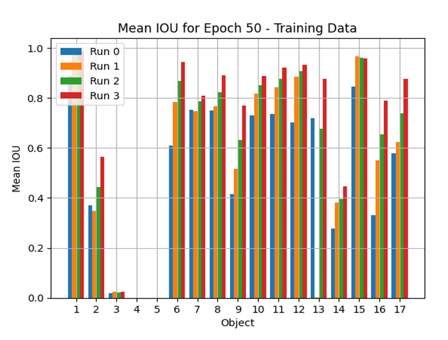Figure 18: Training data.

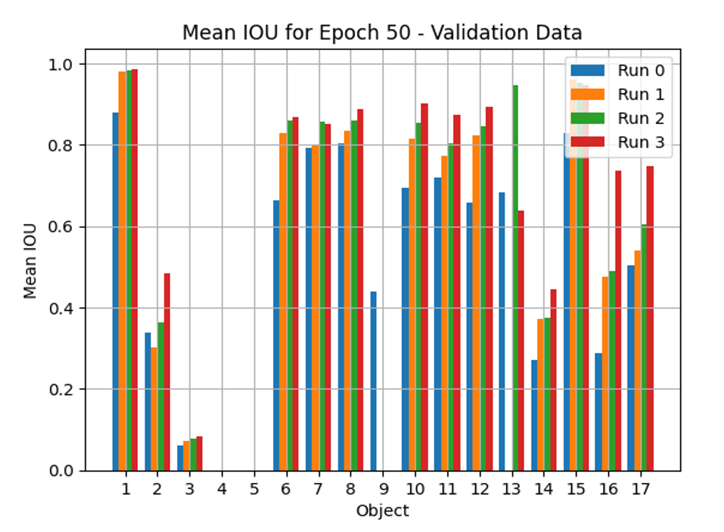Figure 19: Validation data.